One possible explanation for familial aggregates is common exposure to environmental factors; however, such a postulate (shared environmental factors) usually proves unsustainable. Given differences of several decades, it is unlikely that parents and offspring will be exposed to exactly the same deleterious agents. Only if more than one generation is raised in the same house is the hypothesis worthy of serious discussion. Moreover, even if multiple siblings are similarly exposed to a causative agent, one would expect all siblings to be affected rather than only a minority.

Genetic factors are far more plausible. Data from twin studies offer the most overt evidence for existence of genetic factors. Monozygotic (MZ) twins are much more likely to be concordant for any given anomaly (or adult-onset disorder) than are dizygotic (DZ) twins. MZ and DZ twins are generally exposed to the same intrauterine environmental factors; thus, genetic factors need to be invoked.

Familial resemblances for anatomic characteristics are influenced by not one but several genes that cumulatively can produce enough genotypes to mimic a normal distribution in the general population. To illustrate this, let us consider the result of sequentially increasing the number of genes influencing a given trait.

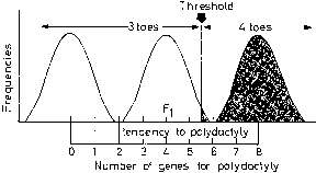
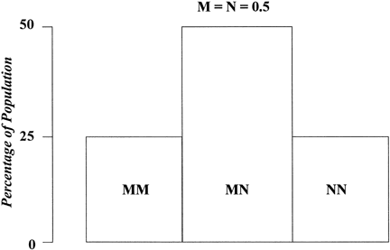
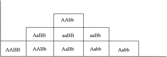
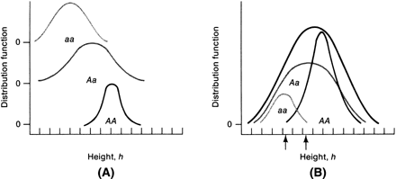
Suppose only one gene controls a given trait and that this gene has only two alleles (A,a). If the frequency of allele A equals the frequency of allele a, 25% of the population is AA based on Hardy-Weinberg equilibrium: p = q = 0.5; p² = q² = 0.25; the frequency of aa is also 25%. Aa accounts for 50% (2 pq = 0.50) (Fig. 1). Now suppose that not one but two genes influence a given trait. At the second locus, alleles B and b exist. Nine genotypes are now possible: AABB, AABb, AAbb, AaBB, AaBb, Aabb, aaBB, aaBb, and aabb (Table 1). The population will contain nine phenotypic classes if alleles A, B, a, and b each exert dissimilar influences. If alleles A and B or a and b exert equal effect, only five phenotypic classes exist (Fig. 2). As the number of genes controlling a trait increases, the number of genotypes in the population increases geometrically. If three genes exist, each with two alleles, there are 27 genotypic classes (3ⁿ). Even more genotypes exist per locus if the locus has more than two alleles. If there is one locus with three alleles per locus, there are 6 genotypes (Table 2). If there are 2 genes, each with 3 alleles, there are 36 genotypes (see Table 2).

Table 1. Relationship Between Numbers of Genes Controlling a Trait and Numbers of Genotypes in a Population

Table 2. Relationship Between Numbers of Genes Controlling a Trait and Number of Genotypes in a Population

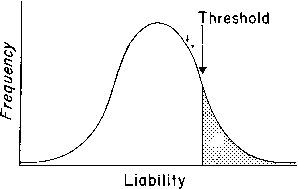
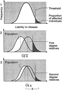
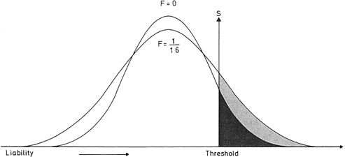
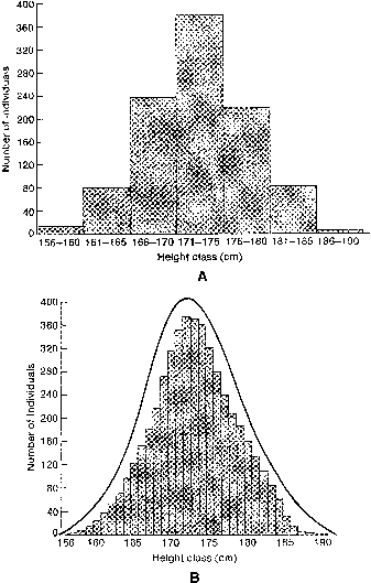
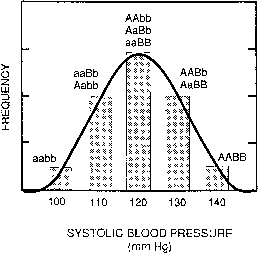
If one histographically represents the number of individuals in each genotypic class, a normal distribution is increasingly approximated as more genotypes exist. With only a few genes, 27 or 36 different genotypes can be produced (see Tables 1 and 2), enough to mimic continuous variation. Figure 3 shows this concept in a different way. If one stratifies heights in the general population into increasingly smaller intervals (1 cm vs 5 cm), histographic representation of the phenotypes better fits the normal distribution. Figure 4 illustrates this for these pathologic traits, the assumption being that only two genes, each with two alleles, determine blood pressure. Table 3 lists several physiologic or anatomic variables for which polygenic inheritance with continuous variation can plausibly be assumed. See Simpson and Elias¹ for additional examples.

Table 3. Anatomic and Physiologic Traits Showing Continuous Variation and Presumably Inherited in Polygenic Fashion

  Age of menarche
  Age of natural menopause (oocyte pool)
  Blood pressure during pregnancy
  Gestational length
  Height
  Pelvic shape
  Resistance against pelvic relaxation
  Responsiveness to medications
  Weight (tendency toward obesity)

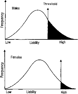
Ostensibly normal distribution of phenotypes in the population can also be explained by several alleles or several genes having nonoverlapping distributions. If only the phenotype is measured, not individual alleles or genes, a normal distribution is seen in the general population (Fig. 5).

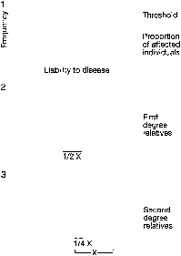
Applying the principles of polygenic inheritance explains why offspring usually, but do not always, reflect parental phenotype. Height can serve as a hypothetical example, for it is well established that a child's height correlates with his/her midparental height, corrected for sex. Suppose height is governed by three genes, each with only two alleles (A,a; B,b;C,c). Each upper case allele (A, B, C) might confer an additional 3 inches in height above some threshold, hypothetically here 60 inches for males and 54 inches for female. Each lower case allele (a, b, c) might contribute nothing above the threshold. Thus, a male of genotype AaBBcC would be 72 inches tall [60 + (4 × 3) = 72]; a female of genotype AaBbCc would be 63 inches tall [54 + (3 × 3) = 63]. On average, one would expect the male parent in the above example to contribute 2 upper case alleles (4/2 = 2) and the female parent 1.5 (3/2 = 1.5). Thus, a child will on average inherit 3.5 upper case alleles and thus approximate parental heights. Offspring, however, could inherit between 1 and 6 upper case alleles and, hence, show heights ranging from 63 to 78 inches in males and 57 to 72 inches in females. The likelihood of various genotypic possibilities producing these extremes is illustrated in Table 4.

Table 4. Hypothetical Example Showing Probability of an Uncommon Genotype (Tall Stature or Short Stature) Arising from a Mating Involving Two Parents of Average Height

Murphy and Chase,² Griffiths and associates,³ Vogel and Motulsky,⁴ and Lynch and Walsh⁵ provide more detailed and mathematically substantiated discussion of the underlying basis of polygenic inheritance.

The term polygenic inheritance is typically used synonymously with continuous variation, but the latter may theoretically result from presence of interaction between a single locus and environmental factors. The environmental factor would presumably need to be almost ubiquitous, but this is not impossible. Examples might include a hazardous waste site, common workplace exposure of low toxicity, or frequently consumed drug (e.g., aspirin) or toxin (e.g., alcohol or cigarette smoke). If environmental as well as genetic factors influence a trait, the term multifactorial is more appropriate.

In humans, one probably cannot distinguish polygenic from multifactorial inheritance, although comparisons between MZ and DZ twins theoretically permit such a distinction. Some geneticists often apply the term polygenic to any trait whose inheritance is complex. Others apply the term multifactorial equally indiscriminately. To this author, it is preferable to invoke the term polygenic/multifactorial, given that the genetic complexities in humans have not been precisely elucidated.

In discontinuous variation, the population consists of two discrete groups. An individual is either affected (e.g., cleft palate) or not. Either an infant has anencephaly or he/she does not. There is no continuum in the population. Table 5 lists several anatomic defects in which discrete affected/unaffected groups exist. In those malformations, the recurrence risk for first-degree relatives is 1% to 5%. Heritable factors of a polygenic/multifactorial nature must exist, or the recurrence risk would not exceed population incidence, which is usually 0.1% or less. To explain the dichotomy (discontinuity) on a polygenic/multifactorial model, one can postulate a threshold beyond which the accrued genetic liability for developing a specific trait becomes so great that a malformation is or can be manifested (Fig. 6). The validity of this concept has been appreciated for at least 70 years. Figure 7 shows results of a 70-year-old landmark breeding experiment in which Wright⁶ found a threshold effect for polydactyly (4 toes) in guinea pigs.

Table 5. Polygenic/Multifactorial Traits Showing Discontinuous Variation

  Cardiac defects (most types)
  Cleft lip (alone)
  Cleft lip, with or without cleft palate
  Diaphragmatic hernia
  Hip dislocation
  Hypospadias (penile or glandular)
  Incomplete Müllerian fusion
  Limb reduction defect (most forms)
  Müllerian aplasia
  Neural tube defects

  (anencephaly, spina bifida,encephalocele)

Phenotypically normal parents delivering a child with a polygenic/multifactorial trait (anomaly) can be assumed to have genetic liabilities nearer the threshold than others in the general population. The small arrows in Figure 6 connote probable genotypes of unaffected parents who have a child with a polygenic/multifactorial trait. Their genotypes are probably nearer the threshold, explaining the higher risk for recurrence in subsequent progeny. By similar reasoning, a parent with a polygenic/multifactorial trait has a 1% to 5% risk for an affected offspring. The risk is less for second- and third-degree relatives than for first-degree relatives because their genotypes are further from the threshold, closer to the mean, for the general population (Fig. 8).

The threshold model becomes highly plausible biologically if “liability”on the abscissa is replaced with “rate of embryonic growth.” If growth is too slow to permit a key embryonic step from being accomplished by a certain time interval, anomalous development may result. For example, if the paired palatine shelves reach the midline prior to a certain day of development, fusion occurs to form the secondary palate. After that day, the shelves are too widely separated to fuse, resulting in cleft palate. In a polygenic model, the inherited factors (genes) might include velocity of growth, size of the mandible and tongue, and rapidity of palatine migration. Similar reasoning could apply to incomplete müllerian fusion or müllerian aplasia.

Certain characteristics are expected of a trait inherited in polygenic/multifactorial fashion and showing discontinuous variation. Traits fulfilling most or all of these criteria can be deduced to be inherited in polygenic/multifactorial fashion, and recurrence risks of 1% to 5%counseled even in the absence of empiric data. These disorders usually have incidence of about 1 per 1000 live births. They typically involve a single organ system or embryologically related organ systems.

Recurrence Risk as Function of Relatedness

In polygenic/multifactorial inheritance, frequency of similarly affected co-twins (concordance) is higher among MZ than DZ twins. Unlike expectations for Mendelian traits, however, discordantly affected co-twins are observed among MZ twins. Table 6 contrasts concordance in MZ and DZ twins for Mendelian versus polygenic/multifactorial inheritance.²

Table 6. Concordance in Twins for Various Modes of Inheritance

Not often appreciated is that consanguineous unions carry increased risks for polygenic/multifactorial traits (Fig. 9). The effect is less pronounced than for autosomal recessive traits. Nonetheless, there are increased risks whenever a common ancestor confers identity by descent of certain alleles, normal or abnormal (Mendelian or polygenic).

Recurrence Risk as Function of Prior Offspring

Unlike Mendelian inheritance, recurrence risk increases empirically after more than one progeny is affected. The risk rarely approaches the 25%expected for recessive traits or the 50% expected for dominant traits;however, after three affected offspring, the risk may be so high (15% to 20%) that one cannot exclude autosomal recessive inheritance in that family.

Recurrence Risk by Severity

The more serious the defect, the higher the recurrence risk. Bilateral cleft palate carries a higher recurrence risk than unilateral cleft palate. Long-segment aganglionosis (Hirschsprung disease) carries a higher recurrence risk than short-segment aganglionosis. Complete uterine didelphysis with vaginal septum should confer a higher recurrence risk than acute or subseptate uterus. Presumably a more severe phenotype indicates genotypic liability further beyond the threshold than is necessary to manifest a less severe trait. In turn, the distribution of genotypes in first-degree relatives (parents) would be more likely to be displaced to the right (i.e., further from the mean of the general population and perhaps just short of the threshold).

Recurrence Risk by Sex

If the trait occurs more frequently among members of one sex, the risk of recurrence is higher if the proband (index case) is of the less frequently affected sex. The prototypic example is pyloric stenosis, which occurs more frequently in men. Thus, the recurrence risk is higher if the proband is female (Table 7). The converse is true for congenital hip dislocation, in which women are more frequently affected. The assumption is that the threshold must be displaced further to the right in the less frequently affected sex, thus resulting in a lower recurrence risk. Figure 10 illustrates this concept.

Table 7. Differences in Recurrence Risks for Pyloric Stenosis

In theory, the exact proportion of genetic and nongenetic factors responsible for multifactorial traits (as strictly defined) can be determined. This proportion is termed heritability (h²). The specific part of variation being estimated quantitatively is additive genetic variation. Additive factors are those that can always be transmitted from generation to generation. The concept of heritability is applied in plant and animal breeding, species in which matings and environment may be controlled.

That heritability measures additive genetic variation means excluding genetic variation independent of dominance or epistasis. Dominance involves interaction between alleles at a single locus, whereas epistasis involves interaction of alleles at different loci. Dominance and epistasis are not additive because their contributions are determined again each successive generation. By contrast, additive factors are always transmitted from generation to generation.

In humans, attempts have been made to calculate heritability for continuous variables such as height or blood pressure. Usually twin studies are used to make estimates; however, in human populations neither matings nor environment can be controlled. Thus, heritability calculations can represent only approximations. The phenomenon actually being calculated in humans is more appropriately called genetic determination. This broader term connotes not only additive genetic factors but also dominance and epistasis. Formally estimating the degree of genetic determination (H) is based on the variance (V) of the differences between MZ and DZ pairs. The formula is

H= V_DZ- V_MZVDZ.

Chromosomal region(s) that co-segregate with a polygenic trait can be identified through linkage analysis. Once theoretically possible but impractical, this approach has now become facile, albeit still laborious, through availability of polymorphic DNA loci. A common finding has been that often a single gene proves to have a major effect, with several additional genes having lesser effects. A search using linkage and clinical features might show etiologic heterogenity. Table 8 shows a hypothetical example of what might become possible. Stratification into various subtypes might permit a precise and more efficacious empirical regimen to be selected. Disorders for which this stratification might be applicable in gynecology include endometriosis, leiomyomata, polycystic ovarian disease, and the common pelvic cancers (e.g., adenocarcinoma of the endometrium, serous or mucinous ovarian epithelial cancer).

Table 8. Hypothetical Example of a Common Disorder Stratified into Three Distinct Subtypes

Performing a genome wide scan to establish candidate regions is known as quantitative trait loci (QTL) analysis. Typically, genotyping is performed using polymorphic DNA markers spaced 10 cM apart. Figure 11 shows idealized results. In the illustration, the chromosomal region between the CAG⁽ⁿ⁾ and the CAT⁽ⁿ⁾ trinucleotide polymorphisms would be worthy of further analysis. Candidate genes within the region(s) identified might be explored through a search of genome databases. Promising candidate gene can be analyzed in more detail by direct (sequencing) or indirect(i.e., single strand conformational polymorphism [SSCP]) methods. The goal is to detect a perturbation (deletion, frameshift, point mutation) in that gene in individuals having the disorder in question.

1. Simpson JL, Elias SE: Genetics in Obstetrics and Gynecology, 3rd ed. Philadelphia, WB Saunders (in press)

2. Murphy EA, Chase GA: Principles of Genetic Counseling. Chicago, Year Book Medical Publishers, 1975

3. Griffiths AJF, Miller JH, Suzuki DT et al: An Introduction to Genetic Analysis, 7th ed. New York, WH Freeman, 2000

4. Vogel F, Motulsky AG: Human Genetics: Problems and Approaches, 3rd ed. New York, Springer-Verlag, 1997

5. Lynch M, Walsh B: Genetics and Analysis of Quantitative Traits. Sunderland, MA, Sinauer Associates, 1998

6. Wright S: The results of crosses between inbred strains of guinea pigs, differing in number of digits. Genetics 19: 537, 1931

7. Loos R, Beunen G, Fagard R et al: Twin studies and estimates of heritability. Lancet 357: 1445, 2001

8. Carter CO: The inheritance of congenital pyloric stenosis. Br Med Bull 17: 251, 1961